GSC API at Scale: Automating Rank Tracking and Anomaly Detection with Python
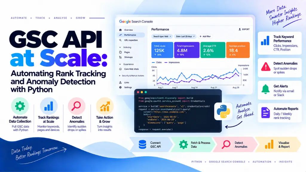

A manual Search Console export works fine for one site with a few hundred keywords. It falls apart once you’re managing multiple properties, need daily granularity instead of a rolling average, or want to know about a ranking drop the morning it happens rather than three weeks later during a monthly review. GSC API at scale means automating the pull, storage, and analysis of Search Console data with Python – and, critically, designing around the API’s hard quotas from the start, since they’re the first wall every team building this hits.
In this article10 sections
This article covers the specific limits that shape any serious GSC automation project, the workarounds teams use in production, and the statistical methods that turn a raw daily pull into an anomaly detection system that flags problems automatically instead of waiting for someone to notice a dashboard looks off.
What Does “At Scale” Actually Mean for the GSC API?#
At scale, in this context, means three things happening simultaneously: pulling data across multiple properties or a large keyword and page inventory, running that pull on an automated daily schedule rather than manually, and layering statistical analysis on top so anomalies surface without a human scanning charts every morning. Each of these compounds the API’s built-in constraints, which is why a script that “works” for a quick one-off pull often breaks down completely once it’s expected to run unattended, daily, across a real site’s full data volume.
The Quota Wall Every Team Hits Eventually#
The Search Console API enforces a set of limits that aren’t negotiable through support requests or higher billing tiers – they apply uniformly regardless of account type.
| Limit | Value | What It Affects |
| Max rows per request (rowLimit) | 25,000 (default is 1,000) | How many rows a single searchanalytics.query call returns |
| Daily row cap per property, per search type | 50,000 rows | Total rows retrievable per day for web, image, or video search separately |
| Short-term load quota | Measured in 10-minute windows | Expensive queries (grouped/filtered by page and query together) can trip this quickly |
| Long-term load quota | Measured in 1-day windows | Persistent over-quota use here requires reducing query complexity, not just waiting |
| Queries per minute | Roughly 1,200 QPM per project | Caps how fast an automated pull can fire requests |
The 50,000-row daily cap is the one that catches most teams off guard, because it applies per property, per search type – not per query. A site with a deep category hierarchy and high query diversity can have most of its actual keyword universe silently excluded from a single day’s pull, since Google fills that allowance sorted by clicks, meaning long-tail, low-volume queries and less-trafficked pages get cut off first. Reported impression loss in real audits has run as high as 67% before applying any workaround – a scale of data loss large enough to make forecasts, cannibalization checks, and content decay analysis built on that data unreliable.
Workarounds for the 50,000-Row Ceiling#
There’s no direct mechanism to raise the standard daily row quota, but several established patterns recover most of the lost data:
- Segment by GSC property. Since the cap applies per property, verifying separate properties for major site sections – by directory path, such as /electronics/ or /blog/ – multiplies your effective daily quota, since each property gets its own independent allowance. Teams running this pattern across dozens of segmented properties have reported cutting impression loss from around 67% down to roughly 11%, capturing over ten times more unique keywords than a single unsegmented pull.
- Query single-day windows rather than long ranges. Requesting one day at a time keeps each query’s load cost lower and reduces the chance of tripping short-term quota limits.
- Avoid grouping by page and query simultaneously. This combination is the most expensive against the load quota; querying by page or by query separately reduces load significantly when both aren’t strictly required.
- Use the BigQuery bulk export for genuinely large sites. Google’s bulk export to BigQuery sidesteps the API’s row and query-level quotas entirely for sites where daily API pulls remain impractical even after property segmentation.
Building the Automated Pull: Pagination and Query Design#
Retrieving more than the default single page of results requires looping through the API’s pagination mechanism, incrementing startRow by the value of rowLimit until a query returns fewer rows than requested – the signal that all available data for that request has been retrieved:
all_rows = []
start_row = 0
row_limit = 25000
while True:
request = {
‘startDate’: start_date,
‘endDate’: end_date,
‘dimensions’: [‘query’, ‘page’],
‘rowLimit’: row_limit,
‘startRow’: start_row,
}
response = service.searchanalytics().query(
siteUrl=site_url, body=request
).execute()
rows = response.get(‘rows’, [])
all_rows.extend(rows)
if len(rows) < row_limit:
break
start_row += row_limit
This loop, run once per property per day and stored in a database rather than re-pulled on demand, is the foundation everything else in an automated pipeline builds on – the same foundational pattern Search Savvy uses when standing up automated reporting for clients managing multiple properties. Running it as a scheduled daily job, rather than pulling a rolling window retroactively, also avoids the API’s tendency to revise recent days’ data slightly as Google finalizes reporting, which can otherwise introduce subtle inconsistencies into a historical dataset.
From Raw Pulls to Signal: Statistical Anomaly Detection Methods#
Once daily data is landing reliably in storage, the next problem is distinguishing a genuine anomaly from normal day-to-day and week-to-week fluctuation. A handful of statistical methods, in increasing order of sophistication, cover most real-world SEO monitoring needs.
| Method | How It Works | Best Fit |
| Rolling z-score | Flags points more than a set number of standard deviations from a rolling mean | Simple metrics with limited seasonality; good default starting point |
| STL decomposition + residual threshold | Splits the series into trend, seasonal, and residual components, then flags large residuals | Metrics with strong weekly or monthly seasonality, which most organic traffic exhibits |
| Isolation Forest | Unsupervised, isolates outliers by recursively partitioning the data without assuming a distribution | Multivariate anomaly detection across several metrics or dimensions at once |
| Median Absolute Deviation (MAD) | Similar to z-score but more robust to the outliers themselves skewing the baseline | Noisy, spiky metrics where standard deviation itself gets distorted by prior anomalies |
A rolling z-score is the right starting point for most teams: fast to implement, easy to explain to a non-technical stakeholder, and effective for catching sharp, sudden deviations. Its weakness is seasonality – organic traffic that predictably dips every weekend will trigger false positives against a naive rolling mean unless that weekly pattern is accounted for first. STL decomposition solves this directly by separating out the seasonal component before applying a threshold to what’s left, which is why it becomes the production default once a team’s monitoring runs daily and unattended without generating alert fatigue from expected weekly dips.
Should I Monitor Anomalies at the Site Level or the Query Level?#
Both, but for different purposes. Site-level or property-level monitoring catches broad issues – an indexing problem, a major algorithm update impact, a technical outage – quickly and with less noise. Query-level or page-level monitoring, applied to your highest-value terms specifically, catches narrower but often more actionable problems, like a single high-traffic page losing rank while overall site metrics stay flat enough to hide the drop in an aggregate view.
A Practical Anomaly Detection Pipeline for GSC Data#
- Automate the daily pull first, respecting the quota constraints and pagination pattern above, before layering statistical analysis on top of incomplete data.
- Start with a rolling z-score on site-level clicks and impressions as a fast first-pass alert layer, accepting some seasonal false positives initially.
- Move to STL decomposition once seasonality causes enough false positives to erode trust in the alerts – most sites reach this point within a few weeks of real-world monitoring.
- Segment monitoring by your highest-priority pages and queries, not just sitewide totals, since aggregate metrics can mask a significant drop in a specific high-value segment.
- Set alert thresholds based on business impact, not statistical elegance. A 3-sigma threshold that fires twice a week for a stakeholder to ignore is worse than a slightly looser threshold that reliably gets acted on.
- Log every flagged anomaly with its resolution, building a reference dataset that can eventually support a more sophisticated Isolation Forest or supervised model as the monitoring program matures.
Search Savvy’s technical SEO services build this kind of automated, quota-aware GSC monitoring directly into ongoing client reporting, rather than relying on manual monthly exports that miss both the data volume and the early-warning value a proper pipeline provides.
Common Mistakes in GSC API Automation at Scale#
- Ignoring the 50,000-row daily cap until it silently distorts reporting. Long-tail keywords and lower-traffic pages get cut first, which can make a forecast or decay analysis look more complete than it is.
- Querying by page and query string together unnecessarily. This is the most quota-expensive combination and often isn’t required for the analysis being performed.
- Applying a flat z-score threshold without accounting for seasonality. This generates enough false positives on organic traffic’s natural weekly pattern that teams eventually ignore the alerts entirely.
- Re-pulling recent days repeatedly without accounting for data revisions. Recent Search Console data can shift slightly as Google finalizes reporting, and treating revisions as new anomalies wastes analyst time.
- Monitoring only sitewide totals. Aggregate metrics can stay flat while a specific high-value page or query cluster experiences a real, actionable decline underneath.
The Bottom Line#
Running the GSC API at scale means designing around its quotas from day one, not discovering them after a pipeline is already in production and silently missing most of a site’s long-tail data. Segmenting properties, pacing queries to avoid the most expensive dimension combinations, and layering a seasonality-aware anomaly detection method like STL decomposition on top of a reliable daily pull turns Search Console from a manual monthly report into a genuine early-warning system.
The practical next step is auditing your current GSC data pull for how much of your actual keyword and page inventory is being silently excluded by the 50,000-row cap, before building any anomaly detection layer on top of it. Search Savvy’s website audit services and keyword research services help teams build this kind of quota-aware, statistically grounded monitoring pipeline, so ranking issues surface in hours rather than during the next scheduled review.
Frequently Asked Questions#
What is the biggest limitation when using the GSC API at scale? The 50,000-row daily cap per property, per search type, is the limit most teams hit first. Because Google fills that allowance sorted by clicks, long-tail keywords and lower-traffic pages get excluded first, which can silently distort any analysis built on top of an unsegmented daily pull.
How can I get more than 50,000 rows of GSC data per day? The most common workaround is segmenting a large site across multiple verified GSC properties by directory path, since each property carries its own independent 50,000-row allowance. For very large sites, Google’s bulk BigQuery export sidesteps the API’s row and query quotas entirely.
What’s the best anomaly detection method for GSC data? A rolling z-score is a good, simple starting point, but most production monitoring eventually moves to STL decomposition, which separates trend and seasonal components before flagging anomalies in the residual – this avoids the false positives a naive z-score generates against organic traffic’s natural weekly patterns.
Should I monitor anomalies at the whole-site level or by individual query? Both, for different reasons. Site-level monitoring catches broad issues like indexing problems or algorithm impacts quickly with less noise, while query- or page-level monitoring on your highest-value terms catches narrower drops that aggregate metrics can otherwise mask.
Why does querying by page and query string together cost more quota? Queries grouped or filtered by both page and query string are the most computationally expensive combination against the Search Console API’s load quota. If an analysis only strictly needs one dimension, querying by page or by query separately reduces the load significantly.
Can I automate GSC exports without hitting rate limits? Yes, by pacing requests to stay under the roughly 1,200 queries-per-minute project limit, querying single-day windows rather than long date ranges in one call, and spreading a large automated pull across the day rather than firing all requests in a short burst.